According to Wikipedia (2022), Resource allocation is a plan for using available resources (…), especially in the near term, to achieve goals for the future. Likewise, from an Operations Research perspective, Resource allocation problems involve the distribution of resources among competing alternatives to minimize costs or maximize rewards (Encyclopedia Britannica, 2022). The problems within these descriptions are characterized by three main components: 1) a set of limited resources; 2) a set of demands to be served, each consuming a specified amount of resources; and 3) a set of costs/returns for each demand and resource. Furthermore, if the allocations made in one period affect those in subsequent periods, the problem is said to be Dynamic. Therefore, the challenge is determining how much of each resource to allocate to each demand.
In Academia and Industry, a large number of problems that fall within the resource allocation umbrella including Portfolio Optimization (Figure 1), Inventory Management, and even Fleet management (e.g. Figure 2 - Ride hailing or Figure 3 - Food delivery).
)](/post/20220404-dynamic-resource-allocation_files/figure00a-etoro-interface.jpg)
Figure 1: Portfolio optimization example (image src)
)](/post/20220404-dynamic-resource-allocation_files/figure00b-uber-driver-interface.jpg)
Figure 2: Fleet management example (image src)

Figure 3: Food delivery platforms
This blog post presents a Dynamic Inventory Management Problem in a Blood Management context for a single hospital, where the blood donations and demands are random variables. This problem is exposed within Warren Powell’s book Approximate Dynamic Programming (2011) and extended on its Reinforcement Learning and Stochastic Optimization (2022) book.
The following sections describe the problem, present the problem’s mathematical model, and explore two solutions strategies: 1) Single-period (myopic) optimization and 2) Value Function Approximation (VFA). Finally, the performance of the solution strategies is compared against a Perfect Information solution.
Before starting I need to say that … This blog post is a summary of my learnings while discovering the Approximate Dynamic Programming and Reinforcement Learning (RL) worlds. I hope you (and my future self) find this useful.
Let’s start …
01/ The blood management problem
One of the challenges a hospital faces in its day-to-day operations is to define how to serve scheduled blood demands while considering the available blood inventory and future donations.
Before going into the problem details, it is worth remembering that blood types are characterized by two elements: their blood group (AB, A, B, and O) and RhD (+ or -). Moreover, these two elements define what “Donor” blood type could serve a “Recipient” blood type. The following table shows the feasible substitutions:
| donor/recipient | AB+ | AB- | A+ | A- | B+ | B- | O+ | O- |
|---|---|---|---|---|---|---|---|---|
| AB+ | X | |||||||
| AB- | X | X | ||||||
| A+ | X | X | ||||||
| A- | X | X | X | X | ||||
| B+ | X | X | ||||||
| B- | X | X | X | X | ||||
| O+ | X | X | X | X | ||||
| O- | X | X | X | X | X | X | X | X |
In this particular case, let us imagine a hospital that at the beginning of every week receives the information on blood demands for the scheduled surgeries. Some of these blood demands can be urgent (or not) and some of them require to be served by the same blood type (i.e. no substitution is allowed).
On the other hand, the available blood supply is determined by the amount of blood stored from the previous week (i.e. blood inventory) plus the donations received during the previous week. The following diagram shows a single-week decision diagram:
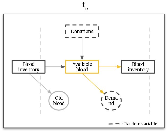
Figure. Single-epoch decision diagram (Yellow arcs highlight our decisions)
Within the previous diagram, the yellow arcs show the available decisions we can make given the available blood supply. Either, we decide to serve a certain amount of demand and/or store some blood for future usage. It is worth mentioning that the blood can’t be stored for an unlimited amount of time and, in our case, its storage is limited to up to 6 weeks. In addition, for simplicity, we will assume all demand doesn’t need to be served, i.e. there are no backlogs for future weeks.
What is our goal?
Blood management might involve costs related to blood storage or spending money to increase donations. However, for this problem, we will try to maximize the doctors’ natural preferences. For example, it is preferred not to substitute blood, or satisfying urgent demand is more important than an elective demand. The next table shows a “monetary” estimation of doctors’ preferences.
Table. Estimated value of doctors’ preferences
| Description | Value |
|---|---|
| Substitution | - $10 |
| O- substitution | $ 5 |
| Filling urgent demand | $40 |
| Filling elective demand | $20 |
| No substitution | $ 0 |
| Holding | $ 0 |
Let’s see an example. Given a \(A+\) elective demand, satisfied with \(O-\) then the total decision contribution would be:
| Substitution: | -$10 |
| Using O-: | +$5 |
| Serving demand: | +$20 |
| Total decision contribution: | +$15 |
In summary, our goal is to maximize doctors’ preferences in the long run considering that every period’s decisions might affect our future alternatives and contribution. The following diagram illustrates this dynamic sequential decision problem.

Figure. Multi-epoch decision diagram
02/ The mathematical model
The underlying analytical problem within the blood management problem is a Dynamic and Stochastic decision problem. It is dynamic because our decisions in a given epoch might affect subsequent decisions, and it is stochastic due to the uncertainty on the blood donations and demand.
This section defines the problem mathematically but without providing a solution strategy/policy to solve the problem. The following section explores the potential solution strategies.
Mathematical formulation
The following formulation is based on Powell (2009)’s modelling framework for dynamic programs. It is composed of the following elements:
- State variables - What do we need to know at time t?
- Decision variables - What are our decisions at time \(t\)?
- Constraints - What constrain our decisions at time \(t\)?
- Exogenous information - What do we learn for the first time between t and t+1?
- Transition function - How does the problem evolve from t to t+1?
- Objective function - What are we minimizing/maximizing and how?
Let’s see them in detail.
Sets
Before defining the State variable, let’s specify the sets:
- \(B\): Set of blood types
(blood_type, age)}: {(A+, 0), (A+, 1), …, (B-, 0), (B-, 1), …, (O-, 6)} - \(D\): Set of demand types plus hold blood for next period (\(d^\phi\))
{blood_type, urgent, substitution_allowed}: {(A+, True, True), (A+, True, False), …, dº}
State variable (\(S_t\))
What do we need to know at time t?
\(S_t=(R_t,D_t)\)
where
- \(R_{tb}\): Units of blood of type \(b \in B\) available to be assigned or held at time \(t\). \(R_t=(R_{tb})_{b \in B}\)
- \(\hat{D}_{td}\): Units of demand of type \(d \in D\) that arose between \(t-1\) and \(t\). \(\hat{D}{t}=(\hat{D}_{td})_{d \in D}\)
Decision variables
What are our decisions at time \(t\)?
\(x_{tbd}\): Number of units of blood \(b \in B\) to assign to demand \(d \in D\) at time \(t\). \(x_t=(x_{tbd})_{b \in B d \in D}\)
Constraints (\(\chi_t\))
What constrain our decisions at time \(t\)?
\[ \sum_{d \in D}x_{tbd} = R_{tb}\qquad \forall b \in B \tag{1} \] \[ \sum_{b \in B} x_{tbd} \leq \hat{D}_{td}\qquad \forall d \in D \tag{2} \]
\[ x_{tbd} \in ℤ_0^+ \qquad \forall b \in B, d \in D \tag{3} \]
Equation (1) states that the sum of all units of blood allocated to all demand types must be equal to the available blood (\(R_{tb}\)) for each blood type \(b \in B\). Equation (2) guarantees that the summation of blood units allocated to a specific demand-type \(d\) must be less or equal to its demand in the current period (\(\hat{D}_{td}\)). Finally, (3) defines the integer nature of the decision variables.
Exogenous information(\(W_{t+1}\))
What do we learn for the first time between t and t+1?
\(W_{t+1} = (\hat{R}_{t+1},\hat{D}_{t+1})\)
where
- \(\hat{R}_{tb}\): Number of new units of blood of type \(b \in B\) donated between \(t-1\) and \(t\).
- \(\hat{D}_{td}\): Units of demand of type \(d \in D\) that arose between \(t-1\) and \(t\).
Transition function (\(S^M(.)\))
How does the problem evolve from t to t+1?
\[ \begin{aligned} S_{t+1} &= S^M(S_t, x_t, W_{t+1}) \\ &= (R_{t+1},\hat{D}_{t+1}) \end{aligned} \]
where \(S^M(.)\) denotes the transition function and depends on the current state \(S_t\), the decision vector \(x_t\), and the exogenous information \(W_{t+1}\).
This function states that \(S_{t+1} = (R_{t+1},\hat{D}_{t+1})\) but to get to this expression we need to also define a how or resource (blood supply) \(R_{t+1}\) evolves, i.e. the Resource transition function. In respect to the demand \(\hat{D}_{t+1}\), there is no need to model its evolution due to it completely depends on exogenous factors.
Resource transition function
\[ \begin{aligned} & R_{t+1} = (R_{t+1b'})_{b' \in B} \\ & R_{t+1b'} = R_{tb'}^x + \hat{R}_{t+1b'} \\ & R_{tb'}^x = f_R^T(x_{tbd^\phi}) \end{aligned} \]
where \(f_R^T(.)\) is the transition function between the number of units held as inventory (\(d^\phi\)) from type \(b \in B\) to the next period’s updated type \(b' \in B\). In our case, this model how the blood ages, i.e. blood age increases +1.
Objective function
What are we minimizing/maximizing and how?
In this problem, the objective is to maximize the summation of the expected total contribution along \(T\) weeks (periods). This can be expressed as
\[ \max_{\pi \in \Pi}\sum_{t \in T}\mathbb{E}[C_t(S_t,X^\pi(S_t))] \] Where,
- \(X^\pi(S_t)\) is a policy that determines \(x_t \in \chi_t\) given \(S_t\).
- \(C_t(S_t,x_t)\) is the total contribution at time \(t\). \[ C_t(S_t,x_t) = \sum_{b \in B}\sum_{d \in D}c_{bd}x_{tbd} \]
Next step
Until this point, the mathematical formulation of the problem was presented but it was never defined how to define our solution strategy (\(X^\pi(S_t)\)). The next section describes some alternative solution strategies and deep dives into two of them.
03/ Solution strategies (policies)
To solve this kind of dynamic problem, multiple approaches can be proposed and explored, for example:
- Tailor-made heuristic
We can design a rule that on every period we assign all the \(O-\) blood units first, and prioritize all the highest reward demand types (i.e. urgent). The 50% remaining blood can be allocated to other demands and the remaining 50% could be stored for the next period. - Single-period optimization
We could solve an optimization problem every week/period to obtain the decisions that maximize the system contribution for a single period without considering the future demand. - Rolling horizon optimization
We could leverage a demand estimation for future periods and solve a deterministic optimization problem not only for the current week but for \(N\) weeks into the future only committing to the current week’s decision. This could be extended to use stochastic programming. - Cost Function Approximation
This policy extends the single-period optimization model by creating additional hard and soft constraints with their respective parameters. For example, adding a penalization for not using old blood that might be lost or not spending more than \(\theta\%\) of the total blood in each period. - Value Function Approximation (VFA)
This policy also extends the single-period aiming to approximate the future contribution of storing units to be used in future periods and solving the single-period optimization problem while considering these estimated future contributions for each blood type.
As the reader can notice, there exist multiple options to solve the same dynamic problem and depending on the problem characteristics one policy can be better than the other. In this blog post, we will only focus on the Single-period optimization and Value Function Approximation and compare their performance.
Single-period optimization
As mentioned before, this policy solves an optimization problem every week only considering the available supply and current demand. Using the notation defined in the previous section, this policy can be defined as:
On every decision period \(t\), our policy is defined as:
\[ X^\pi(S_t) = \underset{x_t \in \chi_t}{\mathrm{argmax}}(\sum_{b \in B}\sum_{d \in D}c_{bd}x_{tbd}) \]
Likewise, we can express this problem as an integer program:
\[ \begin{aligned} & \max \sum_{b \in B}\sum_{d \in D}c_{bd}x_{tbd} \tag{4} \\ & \text{s.t.} \\ & \sum_{d \in D}x_{tbd} = R_{tb}\qquad \forall b \in B \\ & \sum_{b \in B} x_{tbd} \leq \hat{D}_{td}\qquad \forall d \in D \\ & x_{tbd} \in ℤ_0^+ \qquad \forall b \in B, d \in D \end{aligned} \] Equation (4) exhibits the single period objective function which aims to maximize the contribution at a single period \(t\). The Constraints (\(\chi_t\)) are the same defined in the previous section.
Getting our decisions based on this single-period optimization allows us to obtain optimal solutions for a single period \(t\) using linear optimization. Nevertheless, it is worth highlighting that obtaining optimal solutions at every period doesn’t imply an optimal policy in the long run. Therefore, its main drawback is that we aren’t considering any future estimation/information to make our decisions on each decision period.
Value Function Approximation (VFA)
One way to consider the future’s uncertainty within our solution strategy is using a technique named Value Function Approximation (VFA). This technique was inspired by Dynamic Programming and uses as the foundation Bellman’s equations to decompose a large problem into nested subproblems. The main advantage of VFA is that it avoids the (three) curses of dimensionality within dynamic programming. Readers with familiarity with Reinforcement Learning will find this solution strategy quite close to a Q-learning algorithm.
The VFA policy can be expressed as
\[ X^\pi(S_t) = \underset{x_t \in \chi_t}{\mathrm{argmax}}(\sum_{b \in B}\sum_{d \in D}c_{bd}x_{tbd} + \gamma\mathbb{E}[\bar{V}_{t+1}(S_{t+1})]) \]
where
- \(S_{t+1}\) is obtained considering the current state (\(S_{t}\)), the potential decision (\(x_t\)), and the exogenous information (\(W_{t+1}\)), i.e. \(S_{t+1} = S^M(S_t,x_t,W_{t+1})\) .
- \(\bar{V}_{t+1}(S_{t+1})\) is an appropriately chosen approximation of the value of being in state \(S_{t+1}\) at time \(t+1\).
- \(\gamma\) is a discount factor.
In other words, the new term \(\bar{V}_{t+1}(S_{t+1})\) is an approximation of solving the resource allocation problem later in time based on the decision \(x_t\) made at state \(S_t\). However, adding this new term increase the solution complexity and brings some additional challenges.
- Handle an embedded expectation (\(\mathbb{E}\))
- Define a function for value approximation (\(\bar{V}_t\))
- Choose a solution method to efficiently find \(x_t\) on each decision period \(t\)
- Estimate the value of (non-)visited states.
The next sections will address these challenges.
Handle an embedded expectation (\(\mathbb{E}\))
The new expectation (\(\mathbb{E}\)) makes our problem harder to solve. While in a single-period optimization we solve a simple linear optimization problem, the expectation value makes the problem stochastic. To address this issue we could sample scenarios but this can also complicate the optimization problem. However, there is a more elegant approach we could use named post-decision states.
Given that \(S_t\) is the state of the system immediately before making a decision, we can call it the pre-decision state variable,
\(S_t = (R_t, \hat{D}_t)\).
Now, let \(S_t^x\) be the state immediately after we make a decision but before any new exogenous information has arrived, this can be called the post-decision state variable. Therefore, in our case, the post-decision state can be defined as
\(S_t^x=(R_t^x)\)
where \(R_t^x = (R_{tb}^x)_{b \in B}\) is the number of units of blood of type \(b \in B\) held as inventory at time \(t\) to be available on \(t+1\). Notice that the dimensions of the post-decision state are reduced, compared to the pre-decision state, due to we are no longer considering the demand component.
Likewise, if it is possible to define a post-decision state, we can also define a post-decision value function approximation.
Let \(\bar{V}^x_t(S_t^x)\) be the approximated value of being at state \(S^x_t\) after making the \(x_t\) decision.
Using this new concept, it is possible to define our VFA policy as
\[ X^\pi(S_t) = \underset{x_t \in \chi_t}{\mathrm{argmax}}(\sum_{b \in B}\sum_{d \in D}c_{bd}x_{tbd} + \gamma\bar{V}^x_{t}(S^x_{t})) \]
Where,
- \(\bar{V}^x_{t}(S^x_{t})\) is an appropriately chosen approximation of the value of being at state \(S_t^x\).
- \(S_t^x\) is the post-decision state defined as \(S_t^x=(R_{tb}^x)_{b \in B}=(x_{tbd^\phi})_{b \in B}\)
- \(x_{tbd^\phi}\) is the number of units from type \(b \in B\) held as inventory \(d^\phi\) between \(t\) and \(t+1\).
If you want more details about how and why this works, please refer to Powell’s Approximate Dynamic Programming. 2nd Edition - Chapter 4. He provides the details and the logic behind the post-decision states.
Define a function for value approximation (\(\bar{V}_t\))
Lets remember that \(\bar{V}^x_{t}(S^x_{t})\) is an appropriately chosen approximation of the value of being at post-decision state \(S_t^x\). Then, we can define \(\bar{V}_t^x(S_t^x)\) as a separable piecewise-linear approximation.
\[ \bar{V}^x_t(S_t^x) = \bar{V}^x_t(R_t^x)=\sum_{b \in B}\bar{V}_{tb}(R_{tb}^x) \] Where
- \(\bar{V}_{tb}(R_{tb}^x)\) is the scalar piecewise-linear function for blood type \(b \in B\) at time \(t\).
- \(\bar{V}_{tb}(0) = 0\) for all \(b \in B\).
In other words, the approximated value of the post-decision state (\(\bar{V}^x_t(S_t^x)\)) is the summation of the approximated value function for each blood type \(b \in B\) considering \(R_{tb}^x\) units, i.e. \(\bar{V}_{tb}(R_{tb}^x)\) (notice the \(b\) index). Likewise, each of the blood type’s function can be defined as a scalar piecewise-linear function and can be expressed as:
\[ \bar{V}_{tb}(R_{tb}^x)=\sum_{r=1}^{R_{tb}^x}\bar{v}_{tb}(r) \]
It is important to understand that this function is determined by the set of slopes \(\bar{v}_{tb}(r)\) for \(r=0,1, ..., R_{\text{max}}\). where \(R_{\text{max}}\) is an upper bound on the number of blood supply units of a particular type. The following figure shows an example of one \(\bar{V}_{tb}( )\) scalar piecewise-linear function for resource type \(b\). In the figure, it is possible to see that the value of the function depends on the slopes\(\bar{v}_{tb}\).
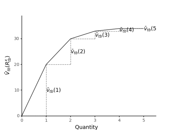
Figure. Scalar piecewise value function (\(\bar{V}_{tb}(R_{tb}^x)\)) for a particular resource type \(b\)
In summary, our value function approximation, i.e. the separable piecewise linear function, instead of directly estimating the value of a given state, will estimate the marginal value (slopes) for each potential number of units for each resource/blood type. Using this approximation has two advantages 1) it is a linear approximation that can be exploited using a linear optimization algorithm, and 2) it is possible to get an estimate of the slope for each type of resource all at the same time (Powell, 2022).
Choose a solution method to efficiently find \(x_t\) on each decision period \(t\)
Based on the post-decision state definition and the separable piece-wise value function approximation, it is possible to model our policy (\(X^\pi(S_t)\)) as a Network Flow problem and solve it using a minimum-cost flow solving algorithm (but aiming to maximize our reward).
The following figures show the network representation of the problem. The first figure shows the network model without the piecewise linear value approximation. It comprises three main layers: 1) Supply blood types nodes (\(R_t\)), 2) Demand nodes (\(D_t\)), and 3) Inventory nodes (\(R^x_t\)). The bold node between the second and third layers is a sink node. The arcs between the first and the second layers represent the potential serving decisions between the supply and demand nodes. Likewise, the arcs between the first and the third layer represent the decision of keeping the blood as inventory for the next period (“hold” decision - \(d^\phi\)). Finally, the arcs between the demand nodes and the sink node determine the maximum amount of blood that could be served for each demand time using the demand value (e.g. \(\hat{D}_{t,\text{AB+}}\)) as the arc upper bound.
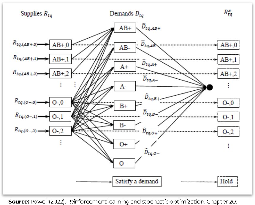
Figure. Policy’s network model without piecewise linear value approximation
In addition, the next figure shows the same network but including piecewise linear value function approximation in a new fourth layer of bold nodes (This new layer is a representation of the rightest super-sink node). The piecewise linear value function approximation is modelled as a set of parallel arcs between the Inventory nodes (3) and the sink node, and the costs of these nodes are defined by the slopes/marginal values (\(\bar{v}_{tb}(r)\)) of the piecewise linear function of each blood type (see the previous section). A simple way to create this modelling trick is to create one arc per each potential inventory unit to be held for future periods, each of these arcs will have its corresponding contribution (\(\bar{v}_{tb}(r)\)) and an upper bound of 1. Finally, given the problem structure, the piecewise linear function is concave; therefore; the slopes of the function are monotonically decreasing, i.e. \(\bar{v}_{tb}(r) \ge \bar{v}_{tb}(r+1)\).
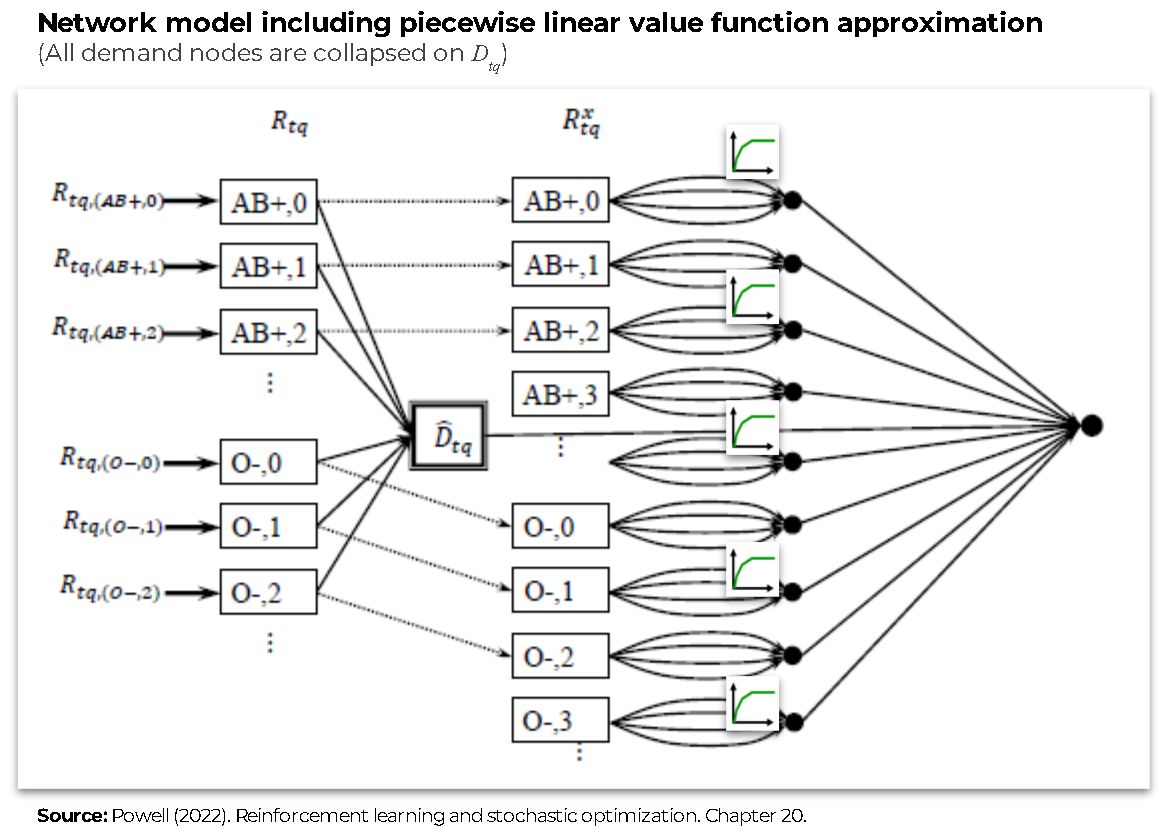
Figure. Policy’s network model with including piecewise linear value function approximation
This network model can be solved easily using a linear programming solver (e.g. CBC, Glop, Glpk, Xpress, Cplex, Gurobi, etc.).
Estimate the value of (non-)visited states.
The previous section described how to use the slopes or marginal values \(\bar{v}_{tb}(r)\) to obtain an approximation of the value function; however, it didn’t define how they are estimated. This section describes how can be leverage sample paths, “exploration” states and the monotonic property of the piecewise linear function’s slopes to estimate the value functions for both visited and non-visited states.
Sample paths
At this stage, it is required to introduce the idea of a sample path denoted as \(\omega\). In short, a sample path refers to a particular sequence of exogenous information. For example in our problem, this could be seen as a scenario of blood demands and donations (it could be either real or simulated). Based on these sample paths, we will be able to get sample realizations of the real value function and use them to refine our value function estimation. For getting multiple samples of the real value function, we can use/generate multiple sample paths (\(\Omega\)).
Exploration states
Let \(S_t^n\) be the pre-decision state variable and \(\tilde{V}_t^n(S_t^n)\), a sample realization of the pre-decision state value at scenario \(n\) within the sample path \(\omega^n\),
\[S_t^n =(R_t^n, \hat{D}_t(\omega^n))\]
\[\tilde{V}_t^n(S_t^n) = \max_{x_t \in \chi_t}(\sum_{b \in B}\sum_{d \in D}c_{bd}x_{tbd} + \gamma\sum_{b \in B}\bar{V}^{x, n-1}_{t}(R^x_{tb}))\]
And let the exploration states be copies of the pre-decision state with a negative or positive perturbation on the available blood units for each resource type,
\[ \begin{aligned} & S_{tb'}^{n-} = ((R_{tb}^n - 1^{b=b'})_{b \in B}, \hat{D}_t(\omega^n)) \qquad \text{for all } b' \in B \quad (\text{if } R_{tb}^n > 0) \\ & S_{tb'}^{n+} = ((R_{tb}^n + 1^{b=b'})_{b \in B}, \hat{D}_t(\omega^n)) \qquad \text{for all } b' \in B \end{aligned} \] where \(1^{b=b'}\) takes the value of \(1\) if \(b = b'\), and zero otherwise.
Therefore, using the same policy (\(X^\pi(S_t)\)) described in the previous section, it is possible to find the exploration state’s value estimations \(\tilde{V}_t^{n+}(S_t^n)\) and \(\tilde{V}_t^{n-}(S_t^n)\) and compute two sample realizations of the marginal values (slopes):
\[ \begin{aligned} & \tilde{v}_{tb}^{n-} = \tilde{V}_t^n(S_t^n) - \tilde{V}_t^n(S_{tb}^{n-}) \qquad \text{for all } b \in B \\ & \tilde{v}_{tb}^{n+} = \tilde{V}_t^n(S_{tb}^{n+}) - \tilde{V}_t^n(S_t^n) \qquad \text{for all } b \in B \end{aligned} \] Finally, using a defined step size (\(\alpha \in (0,1]\)), we can use the slope’s realizations (\(\tilde{v}_{tb}^{n-}\),\(\tilde{v}_{tb}^{n+}\)) to update the slope’s estimation for each blood type’s previous period post-decision state (\(R_{t-1,b_{t-1}}^{x,n}\)).
\[ \begin{aligned} & \bar{v}_{t-1,b_{t-1}}^{n}(r) = (1-\alpha)\bar{v}_{t-1,b_{t-1}}^{n-1}(r) + \alpha \tilde{v}_{tb}^{n-} \qquad \text{if} \quad r = R_{t-1,b_{t-1}}^{x,n} \\ & \bar{v}_{t-1,b_{t-1}}^{n}(r) = (1-\alpha)\bar{v}_{t-1,b_{t-1}}^{n-1}(r) + \alpha \tilde{v}_{tb}^{n+} \qquad \text{if} \quad r = R_{t-1,b_{t-1}}^{x,n} + 1 \\ \end{aligned} \] Notice that \(b\) is indexed with \(t-1\) due to the update step will apply over the previous period blood type attribute before applying the transition function from \(t\) to \(t+1\). For example within our context, if \(b = (A+, 2)\) then \(b_{t-1}\) refers to \((A+, 1)\).
Slopes’ monotonical property
Using the exploration states, we were able to update two of the slopes of the piecewise linear function; however, it is possible that after the update, our function doesn’t hold the monotonic property anymore (i.e. \(\bar{v}_{tb}(r) \ge \bar{v}_{tb}(r+1)\)). This seems like an issue; however, it provides us with the opportunity to update the whole set of slopes with more accurate estimates without exploring all the possible states!!!
In the literature exists multiple approaches to restore the monotonicity of a function. Powell (2022) in Chapter 20 shows three alternatives that he has used. The following figures illustrate one of the approaches using The leveling algorithm.

Figure. Steps of The leveling algorithm. (a) The initial monotone function, with the observed \(R\) and the observed value of the function \(\tilde{v}\); (b) The function after updating the single-segment, producing a non-monotone function; (c) the function after the monotonicity is restored by leveling the function.
The whole VFA algorithm
As the reader can notice, the VFA algorithm requires multiple concepts and merge them together including value function approximation, separable piecewise-linear function, scalar piecewise linear function (based on slopes), pre and post-decision states, sample paths, exploration states and even monotonicity property. Let’s see how to put all of them in a single algorithm.
% This a VFA used to solve the Blood Management Problem
\begin{algorithm}
\caption{VFA algorithm using separable piecewise linear approximation}
\begin{algorithmic}
\STATE  \textbf{Step 0.} Initialization
\STATE $\qquad$ \textbf{0a.} Initialize $\bar{V}_t(S_t^x)$ for all post-decision states $S_t^x$, $t={0,1,...,T}$.
\STATE $\qquad$ \textbf{0b.} Set $n = 1$.
\STATE \textbf{Step 1.} Chose a sample path $\omega^n$.
\STATE $\qquad$ \textbf{Step 2.} Do for $t=0,1,...,T$:
\STATE $\qquad\qquad$ \textbf{2a.} Let the state variable be
\STATE $\qquad\qquad\qquad\qquad$ $S_t^n = (R_t^n, \hat{D}_t(\omega^n))$
\STATE $\qquad\qquad\qquad$ And let the exploration states be
\STATE $\qquad\qquad\qquad\qquad$
        $S_{tb'}^{n+} = ((R_{tb}^n + 1^{b=b'})_{b \in B}, \hat{D}_t(\omega^n)) \quad
        \text{for all } b' \in B $
\STATE $\qquad\qquad\qquad\qquad$
        $S_{tb'}^{n-} = ((R_{tb}^n - 1^{b=b'})_{b \in B}, \hat{D}_t(\omega^n)) \quad
        \text{for all } b' \in B \quad (\text{if } R_{tb}^n > 0)$
\STATE $\qquad\qquad$ \textbf{2b.} Solve
\STATE $\qquad\qquad\qquad\qquad$
        $\tilde{V}_t^n(S_t^n) =
        \max_{x_t \in \chi_t}(\sum_{b \in B}\sum_{d \in D}c_{bd}x_{tbd} +
        \gamma\sum_{b \in B}\bar{V}^{x, n-1}_{t}(R^x_{tb}))$
\STATE $\qquad\qquad\qquad$ Let $x_t^n$ be the decision that solves the maximization problem.
\STATE $\qquad\qquad$ \textbf{2c.}
        Find $\tilde{V}_t^{n+}(S_t^n)$ and $\tilde{V}_t^{n-}(S_t^n)$ using the same policy.
\STATE $\qquad\qquad$ \textbf{2d.} Compute the slopes
\STATE $\qquad\qquad\qquad\qquad$
        $\tilde{v}_{tb}^{n+} =
        \tilde{V}_t^n(S_{tb}^{n+}) - \tilde{V}_t^n(S_t^n)
        \quad \text{for all } b \in B$
\STATE $\qquad\qquad\qquad\qquad$
        $\tilde{v}_{tb}^{n-} =
        \tilde{V}_t^n(S_t^n) - \tilde{V}_t^n(S_{tb}^{n-})
        \quad \text{for all } b \in B$
\STATE $\qquad\qquad$ \textbf{2e.} If $t>0$ update the value function:
\STATE $\qquad\qquad\qquad\qquad$
        $\bar{V}_{t-1}^n=
        U^V(\bar{V}_{t-1}^{n-1}, S_{t-1}^{x,n}, \tilde{v}_{tb}^{n+}, \tilde{v}_{tb}^{n-})$
\STATE $\qquad\qquad$ \textbf{2f.} Update the state variable
\STATE $\qquad\qquad\qquad\qquad$ $S_{t+1}^n=S^M(S_t^n,x_t^n,W_{t+1}(\omega^n))$
\STATE \textbf{Step 3.} Let $n=n+1$. If $n<N$, go to step 1.
\end{algorithmic}
\end{algorithm}
04/ Experimental results
To test the performance of both policies, two instances were defined:
- Epochs(weeks): 15, Max blood age: 3
- Epochs(weeks): 30, Max blood age: 6
For each of the instances, 100 sample paths (simulations) were generated. The exogenous information, i.e. blood demand and donations, in each sample path were modelled as follows:
Demand(blood) ~ Poisson(blood_demand_mean * surge_factor)
  # where "surge_factor" determines randomly increases on demand.
Donation(blood) ~ Poisson(blood_donation_mean)
Finally, to make a fair comparison, the optimal solutions assuming Perfect information were computed for each sample path. Perfection information means that all the future demands and future donations are known.
For more details on the instances and the perfect-information solution model, the reader can check the GitHub repo (mabolivar/blood-management-problem).
Perfect information gap
To obtain a metric to compare both policies, for each sample path, the gap of a policy \(\pi\) was computed as:
\[ \text{gap}^\pi = \frac{\text{reward}^\text{perfect} - \text{reward}^{\pi}} {\text{reward}^\text{perfect}} \]
where \(\text{reward}^\pi\) is the sum of all \(T\) periods contribution (\(\sum_{t \in T}C_t(S_t,X^\pi(S_t))\)) and \(\text{reward}^\text{perfect}\) is the total contribution assuming that all the future demands and future donations are known, i.e. the maximum total contribution in each sample path.
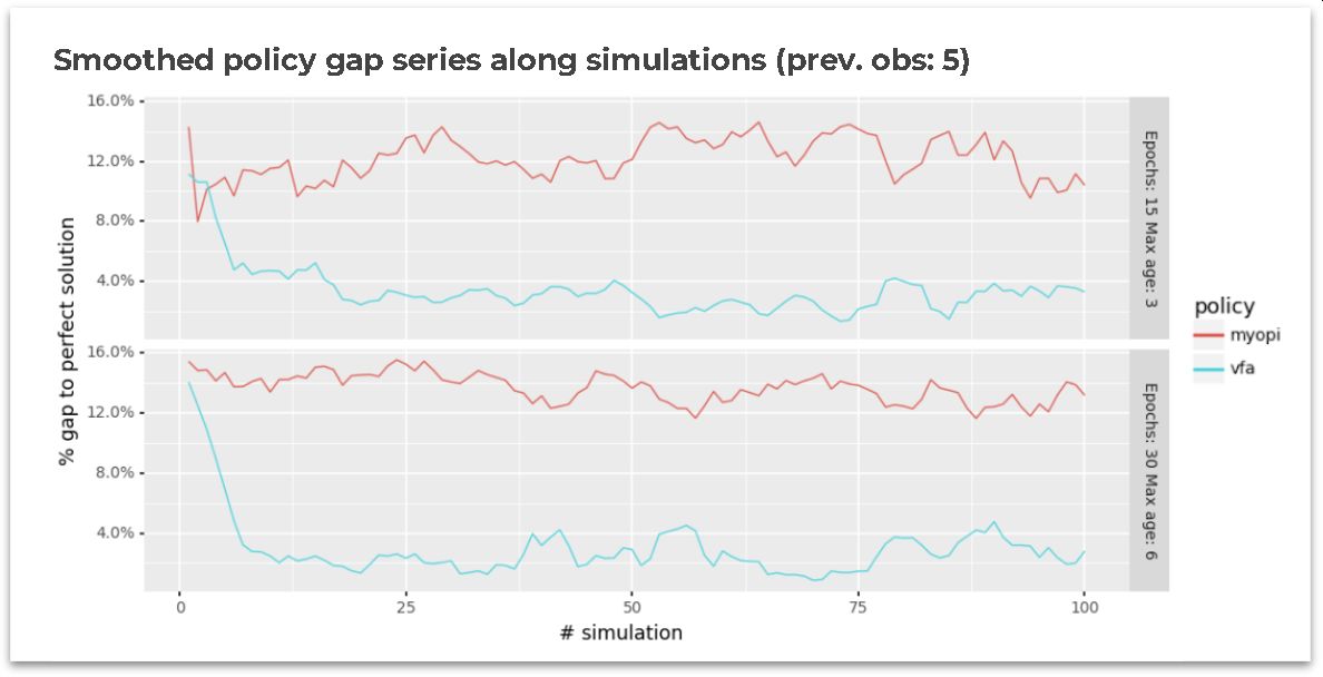
The following table shows average policy gaps compared to the perfect-information solution. The table shows that the single-period optimization has an average gap larger than 12% along with all the simulations. While the VFA policy has an average gap of up to 3.2% compared to the perfect information solution.
| Instance | Single-period (myopic) | VFA |
|---|---|---|
| Epochs: 15 | Max blood age: 3 | 12.2% | 3.2% |
| Epochs: 30 | Max blood age: 6 | 13.7% | 2.7% |
Likewise, the following figure shows the smoothed evolution of the policy’s gaps in both instances. As the reader can notice, the single-period optimization maintains a stable performance among the simulations (as expected). On the other hand, it is possible to see how the VFA policy can “learn” and fastly decrease the gap in the first simulations.
VFA additional gain
Similarly, a reward increase or gain metric was computed comparing the VFA policy against the single-period optimization policy. The following table summarizes the results along with all the simulations. Column 1 states the instance name, and columns 2 and 3 present the average total contribution along with all the simulations for single-period and VFA policies, respectively. Finally, column 4 exhibits the average percentual reward increase for using the VFA policy and the single-period optimization as the baseline. In the last column, it is possible to see that the VFA policy was able to generate more than 10% additional contribution compared to the baseline.
| Instance | Single-period (myopic) Avg.total contribution | VFA Avg. total contribution | Avg. reward increase |
|---|---|---|---|
| Epochs: 15 | Max blood age: 3 | 23,252 | 25,701 | 10.4% |
| Epochs: 30 | Max blood age: 6 | 47,865 | 54,005 | 12.8% |
The next figure shows the smoothed evolution of the additional gain generated by using VFA compared to the single-period optimization policy.
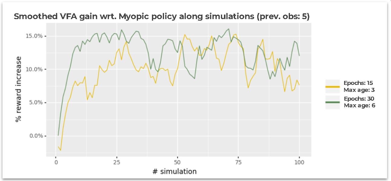
In the first 2-3 simulations, it is possible to see that VFA and single-period optimization have a close performance and in some simulations, the VFA has the worst performance (see the first simulations for Epochs: 15 Max age: 3 instance). However, after those first simulations, the VFA % reward increase significantly rises reaching more than 7% and 12% at simulation # 10 for Epochs: 15 Max age: 3 and Epochs: 30 Max age: 6, respectively. Finally, after simulation #50 the performance oscillates in both instances but maintains an average reward increase of over 10%.
05/ Remarks & Learnings
This was a long journey … (or at least for me)
This blog post started with the definition of the Dynamic Resource Allocation problem and used a Blood Management example to explore two solution approaches (or policies) – Single-period optimization (myopic) and Value Function Approximation (VFA) – but also highlighted that multiple solution approaches exist. Likewise, this blog post covered concepts including the problem’s mathematical model, value function approximation, separable piecewise-linear function, scalar piecewise linear function (based on slopes), pre and post-decision states, exploration states, and even monotonicity property. Finally, it showed the performance of both policies compared to a perfect-information solution plus exhibited the reward increase of VFA with respect to a myopic policy in simulated scenarios.
Based on the time, work and effort in understanding and implementing the previously described elements, these are the main learning I want to share with you:
- Dynamic problem’s challenge is considering the future within the current decision epoch.
Academic literature exposes multiple ways to solve Dynamic problems but the challenge is always the same. Powell provides a great categorization of the four types of solution strategies (policies) for tackling sequential decision problems. Some of the policies consider the future implicitly while others, explicitly. Nevertheless, understanding the four classes helps define a good solution approach. More details about this classification can be found on Castelab’s Sequential Decision Analytics website. - Starting with the problem’s mathematical model provides a reference to explore and define solution strategies/policies.
It is usual for practitioners (like me) to start thinking about the solution approach before understanding the problem to be solved. I found that mathematically modelling the problem – states, decision variables, constraints, exogenous information, transition function, and objective function – helps understanding the problem’s context and could guide to simpler and better solution approaches. - VFA is a strategy that learns while optimizing but it’s more complex compared to other alternatives
As the reader might see, a VFA policy requires to define and control of more elements compared to other policies. However, it has the great quality of “learning while optimizing”. As you might have seen, the policy always provided a decision but at the same time explored other alternative decisions to learn and use that knowledge in the future. - Post-decision states can simplify a problem’s State-space and open the door to new and simple solution methods.
Within the VFA policy, post-decision states gave us the possibility of solving deterministic problems during each decision period. Moreover, using post-decision states with separable piecewise-linear functions allows us to take advantage of deterministic mathematical optimization while solving stochastic problems!. - 💫Not taking an action is also a decision.
Last but not least. After working for some months on this project, I realized that in Dynamic problems, it is not only important to understand the consequences of making a decision but also about not making it. Within the blood management problem, now it might seem obvious that we needed to consider the impact of not allocating the blood for making good decisions (i.e. saving it for the future) – either using VFA or any other policy –. However, at the start of my journey this wasn’t clear and for me was one of the greatest learning.
I hope that you enjoyed and find useful this blog post. If you would like to connect, you can find me on Twitter as @_mabolivar or at Linkedin. I’ll be happy to chat.
Resources
This is a list of some useful resources in case you want to deep-dive more on the topic:
- [Website] Castelab’s Sequential Decision Analytics website
- [Website] ORF 411 - Sequential Decision Analytics and Modeling. Princeton (Slides + Book)
- [Book] Powell (2022). Reinforcement Learning and Stochastic Optimization: A Unified Framework for Sequential Decisions. Wiley.
- [Book] Powell (2011). Approximate Dynamic Programming. Wiley.
- [Paper] Powell (2009) What You Should Know About Approximate Dynamic Programming